Did you ever wonder why newborns pick up so much and so fast of behavior, language, and expressions in just a matter of few years?
Well, the reason is the genetic transfer of DNA and characteristics from parents to offspring. This means that the offspring isn't dumb at all at the time of birth (unlike our machines and ahem..hem AI). It already knows how to catch attention when hungry or smile on seeing familiar faces.
This transfer of intelligence is driven by years of evolution and is hard to match with the current state of Artificial Intelligence.
This explains the difference between human intelligence where a toddler can learn to differentiate between cat and dog just after glancing few images and can even learn more, whereas ML models once trained to identify certain concept can't absorb different concept without forgetting the previous one.
But we can learn something from nature. The transfer of knowledge. Albeit is a different fashion.
Introducing Transfer Learning.
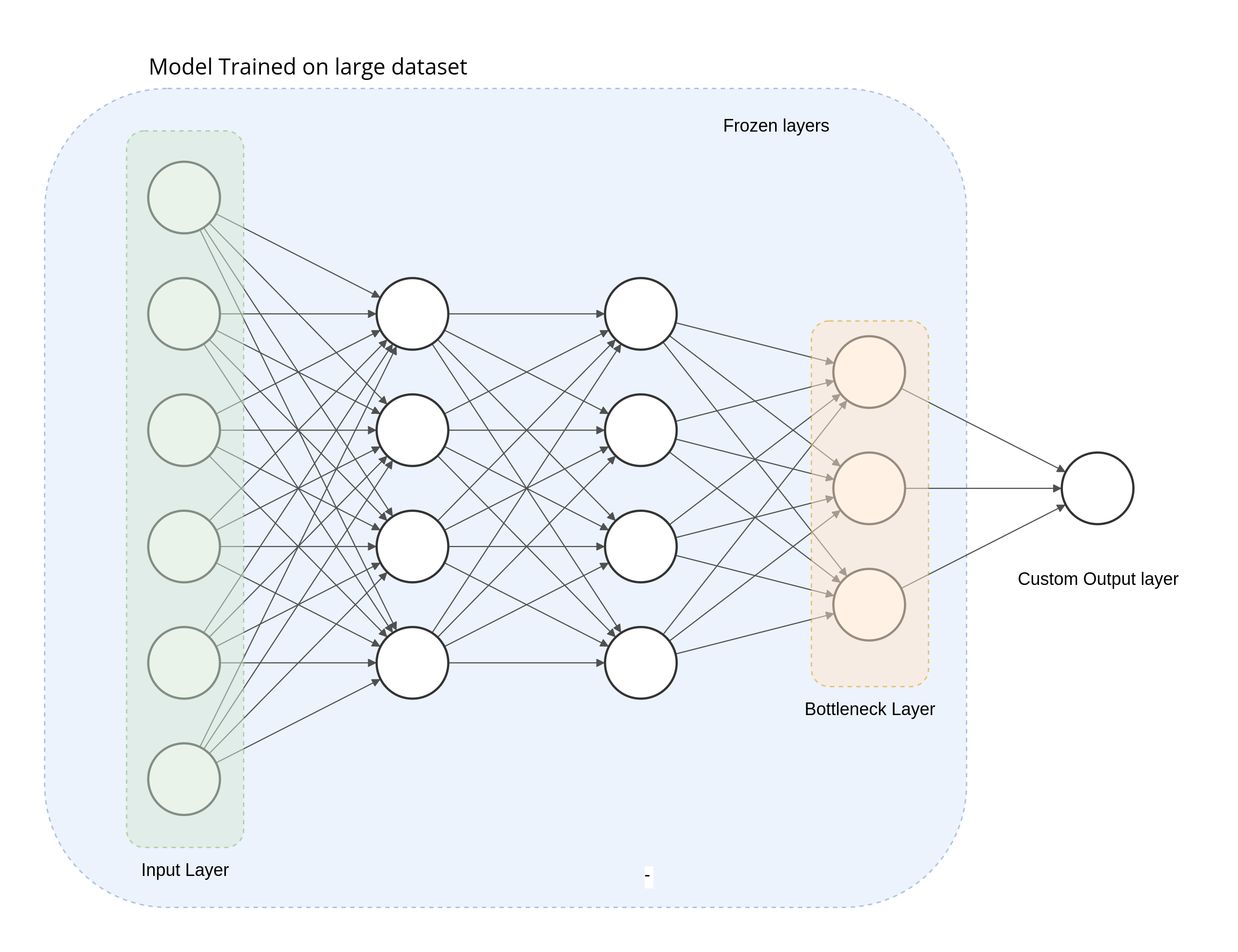
In Transfer Learning, we take part of a previously trained model, freeze the weights, and incorporate these non-trainable layers into a new model that solves a similar problem, but on a smaller dataset.
To go along with the analogy with humans; it's kinda like taking an intellect's brain and fusing it with a toddler one so that the learning can begin where the intellect's ended. Ah, that sounds evil.
But in ML space, it's quite common and not so evil.
Let's take an example. Suppose you are tasked to build an ML model to classify between cats and dogs. If you read through my previous blog post on Checkpoints, we know that the model goes through 3 different phases during training:
- In the first phase, training focuses on learning high-level organization of data.
- In the second phase, the focus shifts to learning the details.
- Finally, in the third phase, the model begins overfitting.
So, even before the model can begin to objectify the concept of cats and dogs, it has to go through the first phase of absorbing high-level organizing of data. That corresponds to making sense of the pixels, their color values, edges, and shapes in the images. This is why we need a huge corpus of data to generalize the high-level concept.
Large image, text datasets like ImageNet (with over 14 million labeled examples) and GLUE can help in many ML tasks and reach high accuracy due to their immense size. But most organizations with specialized prediction problems don't have nearly as much data available for their domain or is expensive to gather, as in the Medical domain where experts are required for an accurate labeling process.
We need a solution that allows us to build a custom model using only the data we have available and with the labels that we care about.
Understanding Transfer Learning
With Transfer Learning, we can take a model that has been trained on the same type of data for a similar task and apply it to a specialized task using our own custom data.
By same of type data, we mean the same data modality–images, text, and so forth. It is also ideal to use a model that has been pretrained on the same type of images. For example, if the end model gets input of cats/dogs from a smartphone camera, use images gathered from a smartphone camera.
By similar task, we're referring to the problem being solved. To do transfer learning for image classification, for example, it is better to start with a model that has been trained for image classification, rather than object detection.
Let's say we are trying to detemine if the given x-ray contains a broken bone or not. As this is a medical dataset, the size is small. Merely, 500 images for each label: broken and not broken. This obviously isn't enough to train a model from scratch, but we can use transfer learning to help a bit. We'll need to find a model that has already been trained on a large dataset to do image classification. We'll then remove the last layer from that model, freeze the weights of the model, and continue training using our 1000 x-ray images.
Ideally, we want the base model to be trained on a dataset with similar images to x-rays. However, we can still utilize transfer learning if the datasets are different, so long as the prediction task is the same. Which in this case is Image Classification.
The idea is to utilize the weights and layers from a model trained in the same domain as your prediction task. In most deep learning models, the final layer contains the classification label or output specific to your prediction task. So, we remove the layerand introduce our own final layer with the output for our specialized prediction task to continue training.
The penultimate layer of the model, the layer before the model's output layer is chosen as the bottleneck layer.

Bottleneck layer
The bottleneck layer represents the inputs in the lowest-dimensionality space.
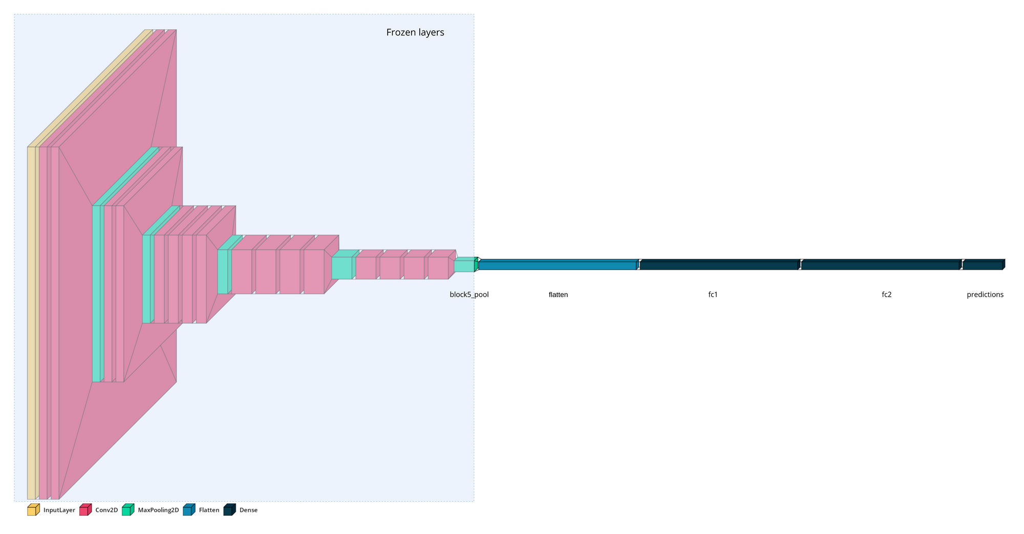
Let's try implementing it in TensorFlow and Keras for X-ray images to detect viral Pneumonia. We are going to use VGG19 pretrained model available in Keras applications module with pretrained weights of imagenet dataset.
vgg_model_withtop = tf.keras.applications.VGG19(
    include_top=true,
    weights='imagenet',
)
Model: "vgg19"
_________________________________________________________________
Layer (type) Output Shape Param #
=================================================================
input_2 (InputLayer) [(None, 224, 224, 3)] 0
block1_conv1 (Conv2D) (None, 224, 224, 64) 1792
... more layer ...
block4_pool (MaxPooling2D) (None, 14, 14, 512) 0
block5_conv1 (Conv2D) (None, 14, 14, 512) 2359808
block5_conv2 (Conv2D) (None, 14, 14, 512) 2359808
block5_conv3 (Conv2D) (None, 14, 14, 512) 2359808
block5_conv4 (Conv2D) (None, 14, 14, 512) 2359808
block5_pool (MaxPooling2D) (None, 7, 7, 512) 0
flatten (Flatten) (None, 25088) 0
fc1 (Dense) (None, 4096) 102764544
fc2 (Dense) (None, 4096) 16781312
predictions (Dense) (None, 1000) 4097000
=================================================================
Total params: 143,667,240
Trainable params: 0
Non-trainable params: 143,667,240
_________________________________________________________________vgg_model_withtop.summary()In this example, we choose the block5_pool layer as the bottleneck layer when we adapt this model to be trained on our Chest X-Ray Images dataset. The bottleneck layer produces a 7x7x512 dimensional array, which is a low-dimensional representation of the input image.
We hope that the information distillation will be sufficient to successfully carry out classification on our dataset.

Since the model we are going to work with accepts images as 224x224x3 dimensional array, we need to either need to resize images to match this model input or change the model's input shape. Here we'll just go with resizing the input image.
vgg_model = tf.keras.applications.VGG19(
    include_top=False,
    weights='imagenet',
    input_shaoe=((224, 224, 3))
)

vgg_model.trainable = False
By setting include_top=False we're specifying that the last layer of the VGG we want to load is the bottleneck layer.
Note that setting include_top=False is hardcoded to use block5_pool as the bottleneck layer, but if we wanted to customize this, we could have loaded the full model, like we previously did, and deleted additional layers.
 block5_conv2 (Conv2D)       (None, 14, 14, 512)       2359808

 block5_conv3 (Conv2D)       (None, 14, 14, 512)       2359808

 block5_conv4 (Conv2D)       (None, 14, 14, 512)       2359808

 block5_pool (MaxPooling2D)  (None, 7, 7, 512)         0

=================================================================
Total params: 20,024,384
Trainable params: 0
Non-trainable params: 20,024,384
_________________________________________________________________
With keras.applications module, by setting input_shape parameter; can change the Layers's dimensions to accomodate for the new input dimension.
Well, do consider that, as a general rule of thumb, the bottleneck layer is typically the last, lowest-dimensionality, flattened layer before a flattening operation.
It is also worth noting that pre-trained embeddings can also be used in Transfer Learning. With embeddings, however, the purpose is to represent an input more concisely. Whereas with Transfer Learning the purpose is to train a similar model, that could be utilized for transfer learning.
Implementing transfer learning
We can implement transfer learning in Keras either by:
- Loading a pre-trained model, removing the layers after the bottlneck layer, and adding a new final layer with our own data and labels.
- Using a pre-trained TensorFlow Hub (https://tfhub.dev) module as the base for your transfer learning task.
Transfer Learning with pre-trained model
We have already set up our VGG model with a bottleneck layer. Let's add a few more layers to make our final model.
from tensorflow import keras

model = tf.keras.Sequential([
    vgg_model,
    keras.layers.GlobalAveragePooling2D(),
    keras.layers.Dense(2, activation="sigmoid")
])
Model: "sequential"
_________________________________________________________________
Layer (type) Output Shape Param #
=================================================================
vgg19 (Functional) (None, 7, 7, 512) 20024384
global_average_pooling2d (G (None, 512) 0
lobalAveragePooling2D)
dense (Dense) (None, 2) 1026
=================================================================
Total params: 20,025,410
Trainable params: 1,026
Non-trainable params: 20,025,410
_________________________________________________________________As you can see the only trainable parameters are from the last layer (after bottleneck layer).
Had we wanted to use our own custom pre-trained model aside from what is offered in keras.applications, we would have done something like this:
model_A = keras.models.load_model("my_model_A.h5")
model_B_ontop_of_A = keras.models.Sequential(model_A.layers[:-1])
model_B_ontop_of_A.add(keras.layers.Dense(1, activation="sigmoid"))model_AAlthough, this method means the model_B_ontop_of_A and model_A shares some weight, and hence when training model_B_ontop_of_A will also affect model_A.
To avoid that, we need to clone the model_A's architecture with clone_model(), then copy its weights (since clone_model() does not clone the weights), and finally freeze the layers:
model_A_clone = keras.models.clone_model(model_A)
model_A_clone.set_weights(model_A.get_weights())

# initialize `model_B_ontop_of_A`
model_B_ontop_of_A = keras.models.Sequential(model_A.layers[:-1])

# Freeze weights
for layer in model_B_ontop_of_A.layers[:-1]:
    layer.trainable = False
Pre-trained embeddings with TF Hub
With TF Hub, we can very easily load a much larger variety of pre-trained models (called modules) as a layer, and then add our own classification layer on top.
hub_layer = hub.KerasLayer(
    "https://tfhub.dev/google/tf2-preview/gnews-swivel-20dim/1",
    input_shape=[], dtype=tf.string, trainable=False
)
And, add additional layers on top:
model = keras.Sequential([
    hub_layer,
    keras.layers.Dense(32, activation='relu'),
    keras.layers.Dense(1, activation='sigmoid')
])
Trade-Offs and Alternatives
Let's discuss the methods of modifying the weights of our original model when implementing transfer learning:
- Feature Extraction
- Fine-tuning
Fine-tuning vs Feature Extraction
Feature Extraction describes an approach to transfer learning where you freeze the weights of all layers before the bottleneck layer and train the following layers on our own data an labels.
In contrast, with fine-tuning we can either update the weights of each layer in the pre-trained model, or just a few of the layers right before the bottleneck.
One recommended approach to determining how many layers to freeze is known as progressive fine-tuning. This involves iteratively unfreezing layers after every training run to find the ideal number of layers to fine-tune. Also, it is recommended to lower down the learning rate as you begin unfreezing the layers.
Typically, when you've got a small dataset, it's best to use pre-trained model as a feature extractor rather than fine-tuning.
| Criterion | Feature extraction | Fine-tuning |
|---|---|---|
| How large is the dataset? | Small | Large |
| Is your prediction task the same as that of the pre-trained model? | Different tasks | Same task; or similar task with same class distribution of labels |
| Budget for training time and computational cost | Low | High |
Is Transfer Learning possible with tabular data?
Tabular data, however, cover a potentially infinite number of possible prediction tasks and data types. And so, as such currently Transfer Learning is not so common with tabular data.
That's all for today.
This is Anurag Dhadse, signing off.


