Deliberately Overfitting your model

Remember those days of your life as an amateur ML enthusiast, celebrating when you trained your model on a toy dataset and received 100% accuracy!

Then you were introduced to the concept of Overfitting.

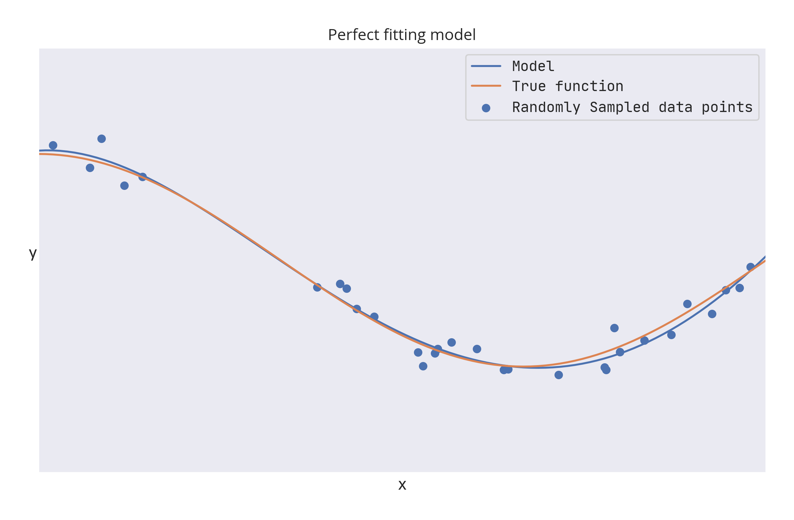
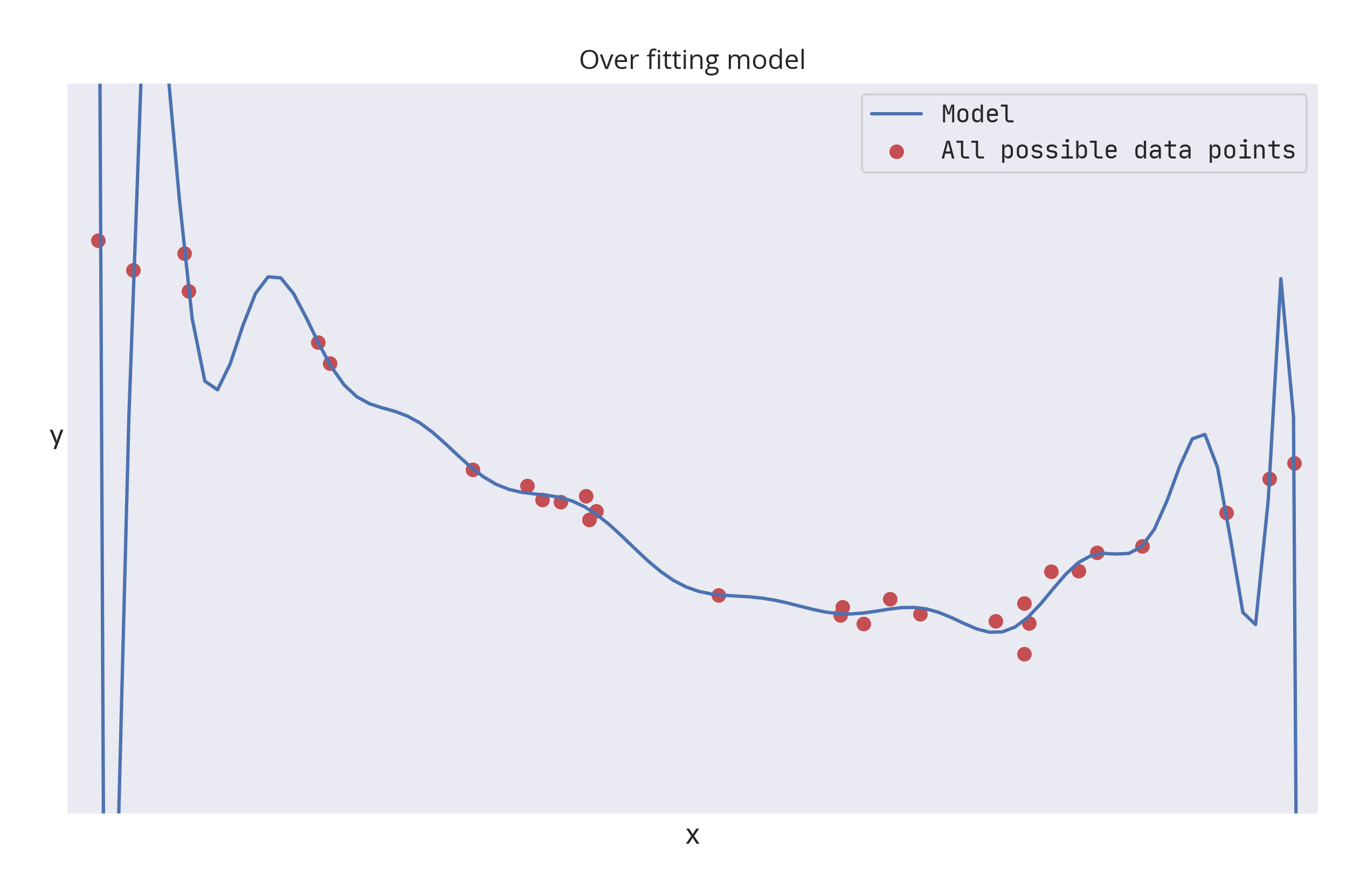
The problem occurs when a model starts to memorize the training data instead of generalizing it to new data. What you wanted was a generalized concept within a model but you got a rote learned model.

But, it's not always that bad. Sometimes you do intentionally want your model to Overfit.

Let's learn when you want to forget about the concept of generalization and accept the fate of rote learning.

The goal of almost all use case scenarios of machine learning is to generalize and learn the overall correlation of features with the label. If our model overfits the training data (the training loss keeps decreasing but the validation loss has started to increase) then the model's ability to generalize suffers and we don't get an effective model.

However, in cases such as simulating the behavior of physical or dynamical systems like those found in climate science, computational biology, or computational finance. These systems are often described by a mathematical function or set of partial differential equations (PDE). Although the equations that govern these systems can be formally expressed, they don't have a closed-form solution, an equation is said to be a closed-form solution if it solves a given problem in terms of functions and mathematical operations from a given generally-accepted set.

Or in other terms, a closed-form expression is a mathematical expression that uses a finite number of standard operations. It may contain constants, variables, certain well-known operations (e.g., + − × ÷), and functions (e.g., nth root, exponent, logarithm, trigonometric functions, and inverse hyperbolic functions), but usually no limit, differentiation, or integration.

For example, the quadratic equation,

$$ax^2 + bx + c = 0$$

is tractable since its solutions can be expressed as a closed-form expression, i.e. in terms of elementary functions (no limit, differentiation, or integration):

$$x=\frac{-b\pm\sqrt{b^2-4ac}}{2a}$$

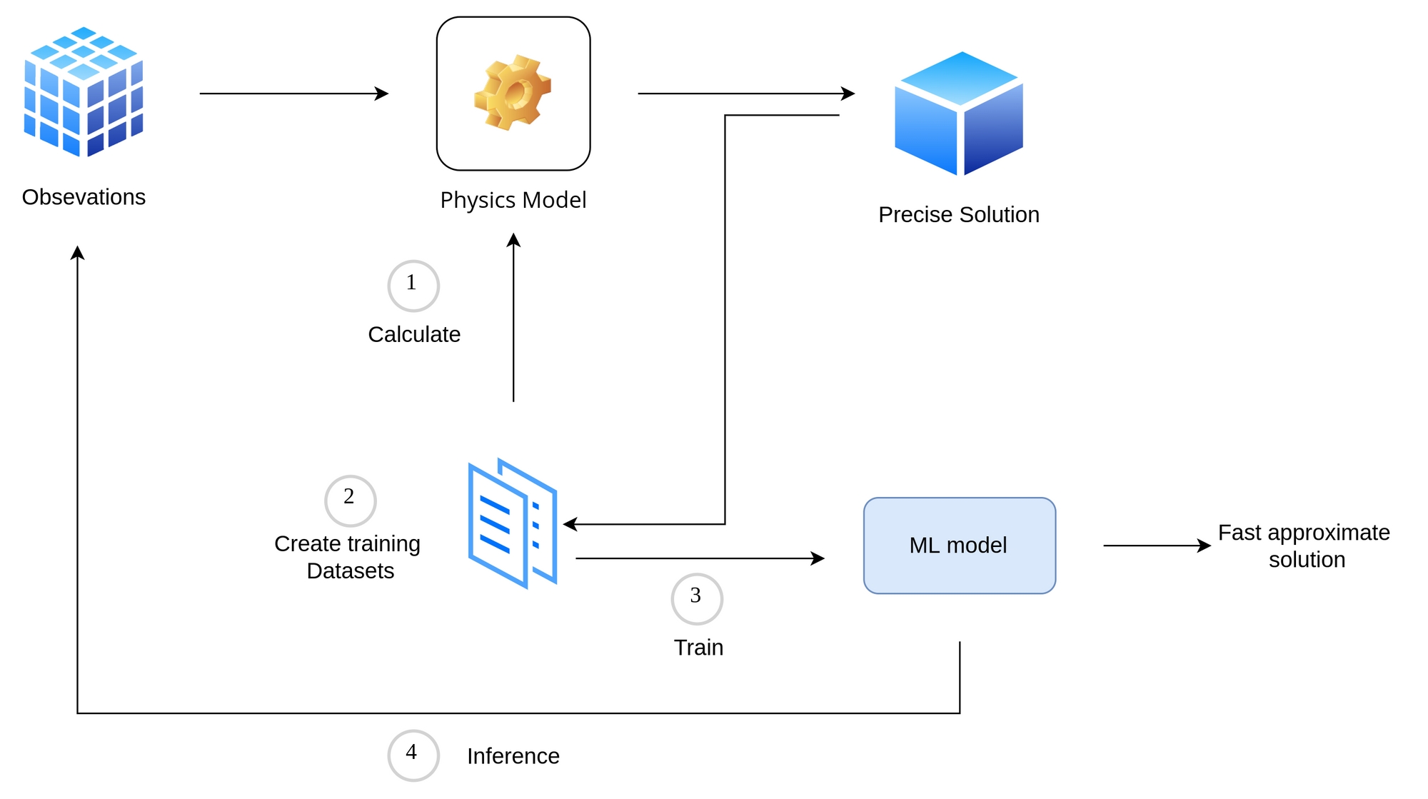
So, these dynamic systems instead use classical numerical methods to approximate solutions. Unfortunately, for many real-world applications, these methods can be too slow to be used in practice.

In such situations, ml models need to learn the precisely calculated and non-overlapping lookup table of inputs and outputs. Splitting such a dataset into the usual training-testing-validation split is also unnecessary since we aren't looking for generalization.

In this scenario, there is no "unseen" data that needs to be generalized, since all possible inputs have been tabulated.

Here, there is some physical phenomenon that you are trying to learn that is governed by an underlying PDE or system of PDEs. Machine Learning merely provides a data-driven approach to approximate the precise solution.

The Dynamic system that we are talking about here is a set of equations governed by some established laws–there is no unobserved variable, no noise, and no statistical variability. For a given set of inputs, there is only one precisely calculated output. Also, unlike other ml problems that suffer from probabilistic nature (like predicting rainwater amount), there are no overlapping examples in the training dataset. For this reason, we don't bother about overfitting our model.

You might ask, why not use an actual lookup table instead of using an ml model in these kinds of situations?

The problem is the training dataset can be too large (in size of Terabytes and Petabytes). Using an actual lookup table is just not possible in production settings. An ml model will be able to infer the approximate solution in a fraction of the time as compared to a lookup table or an actual physics model.

Why does it work?

The usual ML modeling involves training on data points sampled from the population. This sample represents the actual distribution of the data that we want to conceptualize.

When the observation space represents all possible data points, clearly we don't need the model to generalize. We would ideally want the model to learn as many data points as possible with no training error.

Deep learning approaches to solving differential equations or complex dynamical systems aim to represent a function defined implicitly by a differential equation, or system of equations, using a neural network.

Overfitting becomes useful when these two conditions are met,

• There is no noise, so the labels are accurate for all instances.
• You have the complete dataset at your disposal, overfitting becomes interpolating the dataset.

Alternatives and Use cases

Interpolation and chaos theory

The machine learning model we are trying to build here is essentially an approximation to a lookup table of inputs and outputs via interpolation of the given dataset. If the lookup table is small, just use a lookup table, there is no need to approximate it by a machine learning model.

Such interpolation works only if the underlying system is not chaotic. In chaotic systems,  (suffering from probabilistic behavior) even if the system is deterministic, small differences can lead to drastically different outcomes.

In practice, however, each specific chaotic phenomenon has a specific resolution threshold beyond which it is possible for models to forecast it over a short period of time.

So, as long as the lookup table is fine-grained enough and the limits of resolvability are understood, useful approximations via ml techniques are possible.

Distilling knowledge of neural network

Another use case where overfitting comes useful is in knowledge distillation from a large machine learning model where its large computational complexity and learning capacity might not be fully utilized. While smaller models have enough capacity to represent the knowledge, they may lack the capacity to learn the knowledge efficiently.

In such cases, the solution is to train the smaller model on a large amount of generated data that is labeled by the larger model. The smaller model learns the soft output of the larger model, instead of actual hard labels on real data. This is similar to the above discussion, where we are trying to approximate the numerical function of the larger model to match the predictions.

The second training step of training the smaller model can employ useful overfitting.

Overfitting a batch

In the Deep Learning area, it is often preached to start with a complex enough model that can learn the dataset which has the ability to overfit. To generalize such a large model, we then employ regularization techniques such as Data augmentation, Dropout, etc to avoid overfitting.

A complex enough model should be able to overfit on a small enough batch of data, assuming everything is set up correctly. If you are not able to overfit a small batch with any model, it's worth rechecking model code, input and preprocessing pipeline, and loss function for any errors or bugs. This serves as a little checkbox when starting the modeling experimentation.

In Keras, you can use an instance of tf.data.Dataset to pull a single batch of data and try overfitting it:

BATCH_SIZE = 256
single_batch = train_ds.batch(BATCH_SIZE).take(1)

model.fit(single_batch.repeat(),
          validation_data=valid_ds,
          ...)

That's all for today.

This is Anurag Dhadse, signing off.